
Testing an AI-Generated Reversal Strategy, Part 1
Can current generation LLMs create winning trading strategies?

If you listen to the hype, AI can do anything and will take all of our jobs.
I’m still skeptical about that, but I have a lot of respect for the capabilities of current generation large-language models like OpenAI’s GPT-4 and Google’s Gemini. They have their flaws but can achieve incredible results, especially with programming. One recent study found that many programmers are using LLMs for about 50% of their jobs, and I can believe it. LLM code is far from perfect but gives a great starting point to iterate.
I am very, very curious about the quality of trading algorithms LLMs can produce. In theory, LLMs have access to an enormous corpus of trading strategy material. So, I am enjoying the exercise of translating AI-generated trading algorithms to Python and backtesting them.
My first test is on a reversal strategy from GPT-4. I prompted GPT-4 to create a reversal strategy with good risk management, and it generated something we can look at in depth.
I want to start this short series with introductory material. At the end of this post, we will look at a simple backtest on SPY. Our next posts will look at full R2T results.

Introduction to Reversal Strategies
Reversal trading strategies are predicated on the idea that markets move in phases: trends, corrections, and sideways movements. These strategies aim to identify points where a price trend is likely to reverse direction, enabling traders to enter early in a new trend. The core of reversal trading lies in recognizing patterns and signals that indicate the end of the current trend and the beginning of a new one.
The foundation of reversal strategies is rooted in market psychology and supply and demand dynamics. When an asset is overbought, it suggests that buying pressure may soon wane, leading to a potential reversal to the downside as sellers take control. Conversely, when an asset is oversold, selling pressure may be nearing its end, possibly giving way to a reversal to the upside as buyers step in.
The Ichimoku Cloud and the Stochastic Oscillator
We’re using a couple of new indicators here, so I wanted to offer brief explanations. The Ichimoku Cloud in particular is a star of visual storytelling in technical analysis, and I truly enjoy using it. The Ichimoku Cloud provides information on support/resistance, trend direction, momentum, and potential buy/sell signals, all within one chart. Developed by Goichi Hosoda in the late 1930s, the indicator is built on five main components:
Tenkan-sen (Conversion Line): Represents short-term momentum, calculated as the average of the highest high and the lowest low over the last 9 periods.
Kijun-sen (Base Line): Indicates medium-term momentum, derived from the average of the highest high and the lowest low over the last 26 periods.
Senkou Span A (Leading Span A): One of the two lines forming the "cloud", calculated as the average of the Tenkan-sen and Kijun-sen, plotted 26 periods ahead.
Senkou Span B (Leading Span B): The second line of the cloud, determined by the average of the highest high and the lowest low over the last 52 periods, plotted 26 periods into the future.
Chikou Span (Lagging Span): Shows the closing price plotted 26 periods into the past.
The "cloud" is formed between Senkou Span A and Senkou Span B and is the hallmark of the Ichimoku system. Its color (green for bullish, red for bearish) and position relative to the price action provide insight into the market sentiment. A price above the cloud indicates an uptrend, while a price below suggests a downtrend. The cloud's thickness can also signal the strength of the support or resistance it provides.
We’ll be testing this strategy on SPY:

The second indicator is the Stochastic Oscillator. The Stochastic Oscillator is a momentum indicator developed by George C. Lane in the 1950s. It compares a closing price to its price range over a given period, with the premise that momentum precedes price. It oscillates between 0 and 100, with readings below 20 considered oversold and above 80 considered overbought.
The formula consists of two lines: the %K line, which measures current price relative to the high-low range, and the %D line, a moving average of the %K line, acting as a signal line.
This sounds like the RSI, right? The RSI measures the speed and change of price movements to evaluate overbought or oversold conditions. While both indicators aim to identify potential reversal points through overbought and oversold conditions, their calculation methods and interpretations differ. The Stochastics focus on the price's position relative to its high-low range over a period, making it sensitive to price swings and potentially leading to frequent signal changes. This makes it valuable in identifying short-term price reversals and cyclic moves within a trend.
GPT-4’s Reversal Algorithm
After being prompted for a reversal strategy with risk management, GPT-4 offered the following:
Entry Rules:
Bullish Reversal (Buy Signal):The market shows a bullish trend (50-period EMA above 200-period EMA).The Stochastic Oscillator is below 20, indicating an oversold condition.The price is above the Ichimoku Cloud, confirming the bullish sentiment.Enter a buy position when the Stochastic Oscillator crosses back above 20, signaling a potential reversal to the upside.
Bearish Reversal (Sell Signal):The market shows a bearish trend (50-period EMA below 200-period EMA).The Stochastic Oscillator is above 80, indicating an overbought condition.The price is below the Ichimoku Cloud, confirming the bearish sentiment.Enter a sell position when the Stochastic Oscillator crosses back below 80, signaling a potential reversal to the downside.
Exit Rules:
Stop-Loss: Set a stop-loss at 1.5x ATR from the entry point to protect against large losses.Take-Profit: Set a take-profit level at a minimum of 3x ATR from the entry point to ensure a favorable risk-reward ratio.Trend Reversal: Exit the trade if the price moves against the trend direction indicated by the EMA and Ichimoku Cloud alignment.
Results on SPY
Running this algorithm using Python and VectorBT PRO show initially disappointing results. We start with a long/short strategy that includes GPT’s suggested risk management, and our strategy has a win rate of 43% and an expectancy of 0.58. We miss almost all of SPY’s gains for some comparatively low results.
Here is the output from VBT’s portfolio simulator:
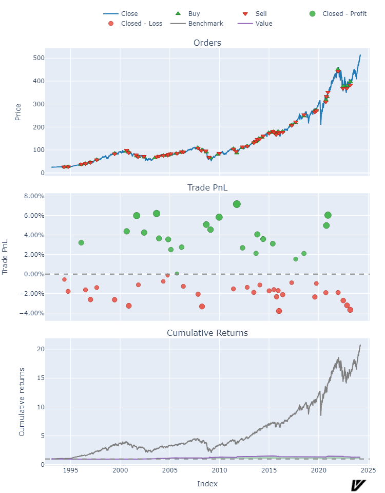
We obviously need to try some iterations! But, we have an interesting start, and in future posts, we will try some parameter configurations as well as variations on the suggested risk management techniques. Just like with programming, I suspect GPT gives us a good starting point, but not a good ending point.
Until next time, keep on the cutting edge, everyone.
Resources
Disclaimers
The content on this page is for educational and informational purposes only. Any views and opinions expressed belong only to the writer and do not represent views and opinions of people, institutions, or organizations that the writer may or may not be associated with.
No material in this page should be construed as buy/sell recommendations, investment advice, determinations of suitability, or solicitations. Securities investment and trading involve risks, and not all risks are disclosed or discussed here. Loss of principal is possible. You are encouraged to seek financial advice from a licensed professional prior to making transaction decisions.
Further, you should not assume that the future performance of any specific investment or investment strategy will be profitable or equal to corresponding past performance levels. Past performance does not guarantee future results.