
Trend Following and Deep Learning, Part 1
Experimenting with neural networks

As we outlined in our introduction post, Alpha on the Edge is part algorithmic trading, part AI experimentation. AI - particularly deep learning - is advancing rapidly, and the finance industry is still trying to find out what works. There are enormous challenges with AI - domain expertise and computational resources being top among them.
This leaves room for a lot of fun experimentation. We can enjoy the excitement of research without the baggage of excessive conventions. Experimentation is about exploration, discovery, innovation - all very fun things.
It’s also about failure.
Behind every shining research result is a heap of failed and aborted tests. That’s not necessarily a bad thing, though. It means experimentation requires iteration, curiosity, and a willingness to get it wrong.
At Alpha on the Edge, we want to both contribute to and be involved in the discourse around AI in finance. We want to share results and code and engage with fellow enthusiasts. We want to show what we’ve gotten wrong and what we’ve gotten …. less wrong?
So that’s what you can expect from our AI posts. Experiment results, good and bad, along with code, discussion, and carefully veiled invectives about programming reflections on the process.
Let’s get started.
Trend Following with CNN-LSTM Deep Learning Models
We start with research from Patrik Eggebrecht and Eva Lütkebohmert (2023). They present results from the innovative use of Convolutional Neural Network (CNN) and Long Short-Term Memory (LSTM) models with trend following.
Before diving into the specifics of the trading strategy, let's unpack the CNN-LSTM model. This model is a fusion of two powerful deep learning approaches: the CNN and LSTM.
CNNs are known for their prowess in extracting spatial features from data. In the context of stock market data, CNNs can discern patterns and features from historical price data, which might indicate a trend or a shift in market sentiment.
LSTMs, on the other hand, are a type of recurrent neural network (RNN) that excel in processing sequences of data. They are particularly adept at remembering long-term dependencies, making them ideal for time-series data like stock prices.
When combined, the CNN-LSTM model harnesses the strengths of both: the CNN extracts relevant features from the data, and the LSTM uses these features to make predictions based on the sequence of data. This hybrid model is particularly well-suited for financial markets, where both spatial patterns and time-series trends are crucial for making accurate predictions.
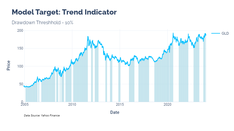
Model Target - Trend Indicator
The research tries to train the model to predict a binary trend indicator. In short, the indicator flags periods when a perfect trader would have caught price increases prior to drawdowns of a given percentage. The drawdown percentage is the only parameter for this indicator.
This shows the indicator for the SPDR Gold Trust (GLD) ETF:
Prediction vs Classification
A quick note on model targets here. Many try to use neural networks for time series value prediction. This has mixed success, but it is easier for many outside the field of deep learning to understand.
I am not completely convinced that prediction is the best way to use deep learning in finance. This model uses binary classification. The raw outputs of the final sigmoid function are in the range [0,1]. These can be interpreted as the “probability” that the model assigns to being in a trend at a given time.
In future posts, I would like to explore prediction vs classification for time series in more depth.
Model Architecture (with code)
The model discussed in the study consists of two 1D convolutional layers, each equipped with 16 filters and a Rectified Linear Unit (ReLU) activation function. The second convolution layer's output then passes through a max pooling layer, which helps reduce the dimensionality of the data and extract the most significant features.
A crucial step follows: the output is flattened to make it suitable for the LSTM layer. This LSTM layer, with 10 hidden memory blocks, captures the temporal dependencies in the data. Finally, the model concludes with three fully connected layers that lead to a single output neuron with a sigmoid activation function. This architecture results in a model with 4959 trainable parameters.
In PyTorch, a basic recreation looks like this:
import torch.nn as nn

class CNNLSTM(nn.Module):
    def __init__(self, input_channels):
        super(CNNLSTM, self).__init__()

        # CNN
        self.conv1 = nn.Conv1d(in_channels=input_channels, out_channels=16, kernel_size=2)
        self.conv2 = nn.Conv1d(in_channels=16, out_channels=16, kernel_size=2)
        self.relu = nn.ReLU()
        self.maxpool = nn.MaxPool1d(kernel_size=3)

        self.dropout = nn.Dropout(0.2)

        # LSTM
        self.lstm = nn.LSTM(input_size=16, hidden_size=10, batch_first=True)

        # Fully connected layers
        self.fc1 = nn.Linear(10, 10)
        self.fc2 = nn.Linear(10, 5)
        self.fc3 = nn.Linear(5, 1)

        # Initialize weight matrices
        nn.init.xavier_uniform_(self.fc1.weight)
        nn.init.xavier_uniform_(self.fc2.weight)
        nn.init.xavier_uniform_(self.fc3.weight)

        # Final activation function
        self.sigmoid = nn.Sigmoid()

    def forward(self, x):
        # CNN layers
        x = self.relu(self.conv1(x))
        x = self.relu(self.conv2(x))

        # Dropout
        x = self.dropout(x)

        # Max pooling
        x = self.maxpool(x)

        # Flattening for LSTM
        x = torch.transpose(x, 1, 2)

        # LSTM
        x, (hn, cn) = self.lstm(x)

        # Select the output of the last LSTM time step
        x = x[:, -1]

        # Apply fully connected layers with ReLU activation and final sigmoid activation
        x = self.relu(self.fc1(x))
        x = self.relu(self.fc2(x))
        x = self.relu(self.fc3(x))
        x = self.sigmoid(x)

return xPreliminary Analysis with PyTorch
I recreated the model with the same feature space used in the study. The researchers used basic technical indicators to create features for each security:
SMA
EMA
RSI
Bollinger Bands
MACD
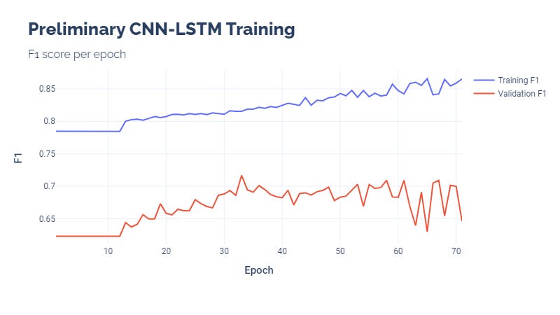
The preliminary analysis used an early stop mechanism that allowed the calibration to run for 15 epochs of no validation increase. This needs to be calibrated further. As it stands, our training loss continued decreasing, which means that the model was learning. The problem is that the results do not generalize quite well.
Our training set used all history of GLD through 2021. 2022 was our validation set, with 2023 being our test set.
Training visualizations:

Test Set Results
Let’s visualize the model’s predicted indicator values using the cutoff with the highest accuracy (0.8):

This is a challenging set for our model because it was a ranging market. Even still, if we had traded this strategy, it would have outperformed GLD (without considering slippage).
Looking Ahead
We have many, many possible avenues to explore here:
Modified CNN-LSTM architectures
Different feature sets
Different parameters
Portfolio strategy using ranked outputs
I would enjoy the chance to hear your comments, as well. What would you like to see? Where do you think we should go with this?
Until next time, keep on the cutting edge, everyone.
References
Eggebrecht, Patrik & Lütkebohmert, Eva. (2023). A Deep Trend-Following Trading Strategy for Equity Markets. The Journal of Financial Data Science. 5. jfds.2023.1.120. 10.3905/jfds.2023.1.120.
Disclaimers
The content on this page is for educational and informational purposes only. Any views and opinions expressed belong only to the writer and do not represent views and opinions of people, institutions, or organizations that the writer may or may not be associated with.
No material in this page should be construed as buy/sell recommendations, investment advice, determinations of suitability, or solicitations. Securities investment and trading involve risks, and not all risks are disclosed or discussed here. Loss of principal is possible. You are encouraged to seek financial advice from a licensed professional prior to making transaction decisions.
Further, you should not assume that the future performance of any specific investment or investment strategy will be profitable or equal to corresponding past performance levels. Past performance does not guarantee future results.