
Testing an AI-Generated Reversal Strategy, Part 2
In AotE fashion, "testing" means over 64 million simulations

Welcome back, everyone, to an experiment in using artificial intelligence via Large Language Models (LLMs) to generate a reversal trading strategy. We asked GPT4 for a reversal strategy with good risk management, hoping that the collective knowledge of the corpus of text GPT4 was trained on could reveal a useful trading strategy.
In our first post on this strategy, we introduced the strategy in broad strokes, discussed the trading rules, and performed an initial backtest on SPY.
In this second post, we will look at a more extensive set of backtests on the stocks in the S&P 500.
You all know how we like to do things around here. We literally did over 64 million simulations to test this strategy. If anyone can be said to have really put an AI’s claim to the test, it’s us.
We will also take a beat to discuss parameter stability and feasible parameter spaces. For a strategy like this, these considerations matter a lot.

Parameter Space
Believe it or not, this strategy has 12 parameters:
Fast MA Window
Slow MA Window
Stochastic K
Stochastic Slow K
Stochastic Slow D
Stochastic Lower Threshold
Stochastic Upper Threshold
Ichimoku Cloud Tenkou
Ichimoku Cloud Kijun
Ichimoku Cloud Senkou
Stop Loss ATR Multiplier
Take Profit ATR Multiplier
The parameter space for this strategy can grow really, really quickly. Even just 3 values per parameter creates a parameter space of over 1 million possibilities, which strains both computational resources and usefulness for such a large parameter space. We limited our test to ~150,000 parameter configurations to give a solid foundation for our results. The parameters all stayed around the “standard” values for the indicators - 9 for the Ichimoku tenkou, etc.
One consideration in backtesting is parameter stability. This can be defined a number of ways, but the idea is simply to help us determine if we are curve fitting or not. If the strategy’s results change dramatically for a change in one parameter, this is evidence that the “optimal” parameter configuration is an anomalous result.
Result Overview
For each stock in the S&P 500 with history available from 2008, we ran simulations for each of the ~150,000 parameter configurations, which gave us over 64 million simulations to look at.
If you take the best metric for each stock, the results look like this:
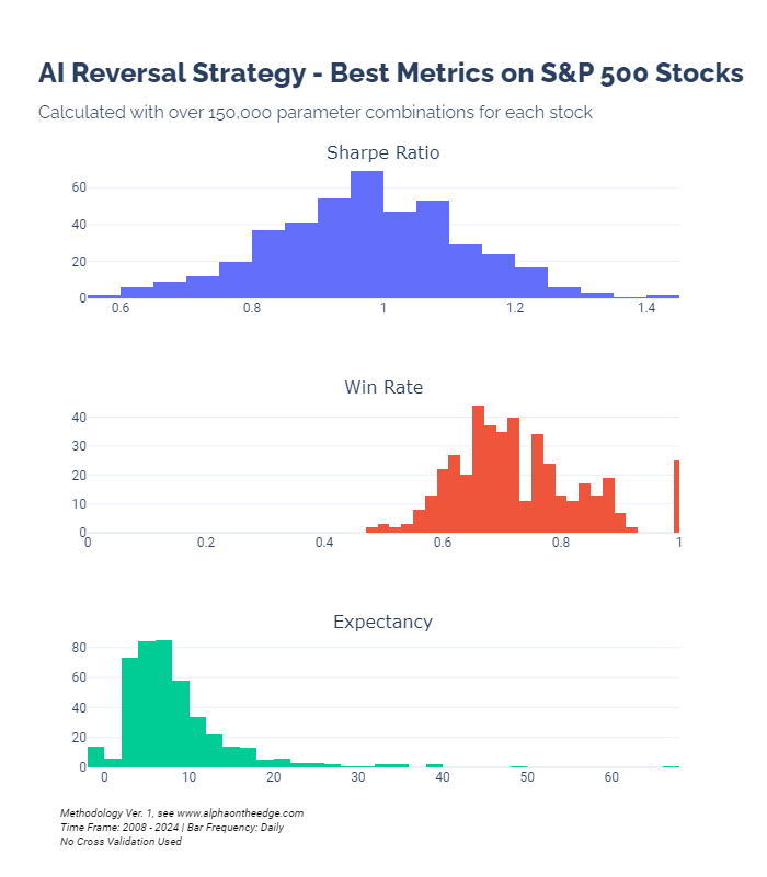
A couple of things stand out - this strategy tends to give favorable win rates. Historically, it has been better than a coin flip for the best parameter configuration on almost every stock tested. That’s impressive.
What’s less impressive are the risk-adjusted performances of the strategy on each stock. Even with the “risk management” prompt, GPT4’s suggested use of ATR-based SL and TP thresholds did not give us incredible Sharpe ratios. They aren’t terrible, though.
Looking at the outlier expectancy values - this strategy happened to catch a few lucky pops on stocks with very few signals. These results filter out simulations with low numbers of trades, but on some of the stocks here, you can expect to see outlier results. That’s why we like to look at medians and distributions!
But About Those Parameters
Let’s return to the topic of parameter stability. Again, defining “stable” parameters is more an art than a science, but our goal is to see if our results are anomalous. If we change the fast MA window 5 bars, say, and the simulation’s performance tanks, that’s not a sign of a robust strategy.
With such a large parameter space, my idea was to take a simple approach. I wanted to look at the simulated Sharpe ratios for 3 sets of simulations:
The optimal parameter configuration for each stock (the values plotted in the histograms above)
The parameter configuration with the highest median Sharpe ratio across all stocks
The parameter configuration comprised of the values most like to be used in the optimal configuration for each stock.
The third set deserves a little more explanation, because I have not seen it used elsewhere. I calculated the probability that each parameter value would be in the optimal configuration for each stock.
For example, we tested 2 different values of the ATR multiple for a stop loss. Of the 432 optimal configurations, 87% of those used a multiplier of 4.0.

One main message here is that as soon as you step out of the “optimal” configuration for each stock, you potentially lose 0.3-0.4 on your Sharpe ratio. This gives some pause for the generalizability of this strategy. Our tests here did not use cross validation, which we might do in the future (the primary obstacle is computing power - 64 million simulations would become 1.2 billion simulations).
Another main message is that this strategy depends on the stock it’s used on. In that vein, here are the 10 stocks with the highest optimal Sharpe ratio from this strategy:

Thanks for checking out our research into this reversal strategy, everyone! The results are promising. We will definitely try more AI-generated strategies in the future. If AI will truly take all of our jobs in the future, we need to know what it can do!
Until next time, keep on the cutting edge, everyone.
Resources
Disclaimers
The content on this page is for educational and informational purposes only. Any views and opinions expressed belong only to the writer and do not represent views and opinions of people, institutions, or organizations that the writer may or may not be associated with.
No material in this page should be construed as buy/sell recommendations, investment advice, determinations of suitability, or solicitations. Securities investment and trading involve risks, and not all risks are disclosed or discussed here. Loss of principal is possible. You are encouraged to seek financial advice from a licensed professional prior to making transaction decisions.
Further, you should not assume that the future performance of any specific investment or investment strategy will be profitable or equal to corresponding past performance levels. Past performance does not guarantee future results.